GSoC 2024 | QGANs for Monte Carlo Simulations

What is Google Summer of Code?

I spent the last summer working in GSoC 2024 with the ML4SCI organization. Google Summer of Code is an international online program designed to introduce new contributors to open-source software development. During this program, GSoC participants collaborate with an open-source organization on a programming project lasting 12 weeks or more under the supervision of mentors. Participating in GSoC was one of the most enriching and challenging experiences of my life. My project, QGANs for Monte Carlo Simulations aims to investigate the feasibility of using Quantum Generative Adversarial Networks to generate events for Monte Carlo simulations. The code of this project is available in Git Hub.

Monte Carlo Simulations

Monte Carlo Simulation is a computational technique that uses repeated random sampling to estimate the probability of various outcomes in uncertain scenarios. Developed by John von Neumann and Stanislaw Ulam during World War II, it is named after the Monte Carlo casino due to its reliance on chance. The method is widely used in finance, project management, and AI for risk assessment and decision-making. It involves setting up a predictive model, specifying probability distributions for input variables, and running several simulations to generate possible outcomes.

Monte Carlo Simulation differs from typical forecasting models by predicting a range of outcomes based on estimated values rather than fixed inputs. It builds a model using probability distributions for variables with inherent uncertainty. By recalculating results repeatedly with different random values, often thousands of times, it generates a wide array of possible outcomes.

Generative Adversarial Networks

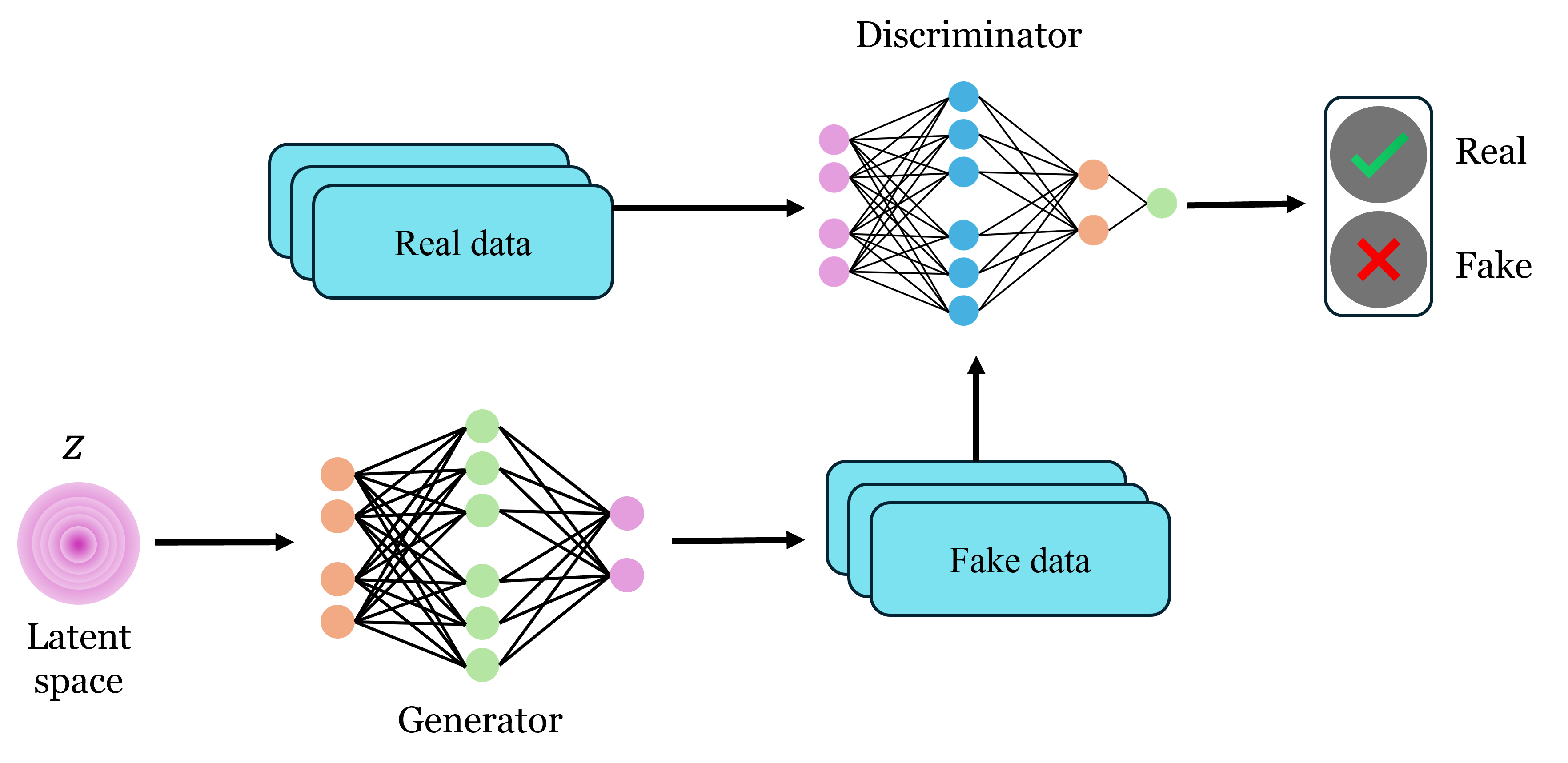
Generative Adversarial Networks (GANs) is a framework for estimating generative models using an adversarial process [1]. This framework involves training two models simultaneously: a generative model \(G\) that captures the data distribution and a discriminative model \(D\) that distinguishes between samples from the training data distribution and those produced by \(G\). The goal is to improve \(G\) so that \(D\) cannot differentiate between training data and generated data. This process is similar to a minimax two-player game, where \(G\) tries to fool \(D\) while \(D\) aims to detect the fake data. We train \(D\) to maximize the probability of assigning the correct label to both the training data samples and the generated samples from \(G\). Simultaneously, we train \(G\) to minimize the chances of \(D\) correctly distinguishing between training and generated samples. This process involves optimizing the loss function:

where \(D(\mathbf{x})\) represents the probability that \(\mathbf{x}\) came from the true data and \(D(G(\mathbf{z}))\) the probability of \(D\) correctly labeling a generated sample \(G(\mathbf{z})\) from the latent space \(\mathbf{z}\).

Quantum Generative Adversarial Networks

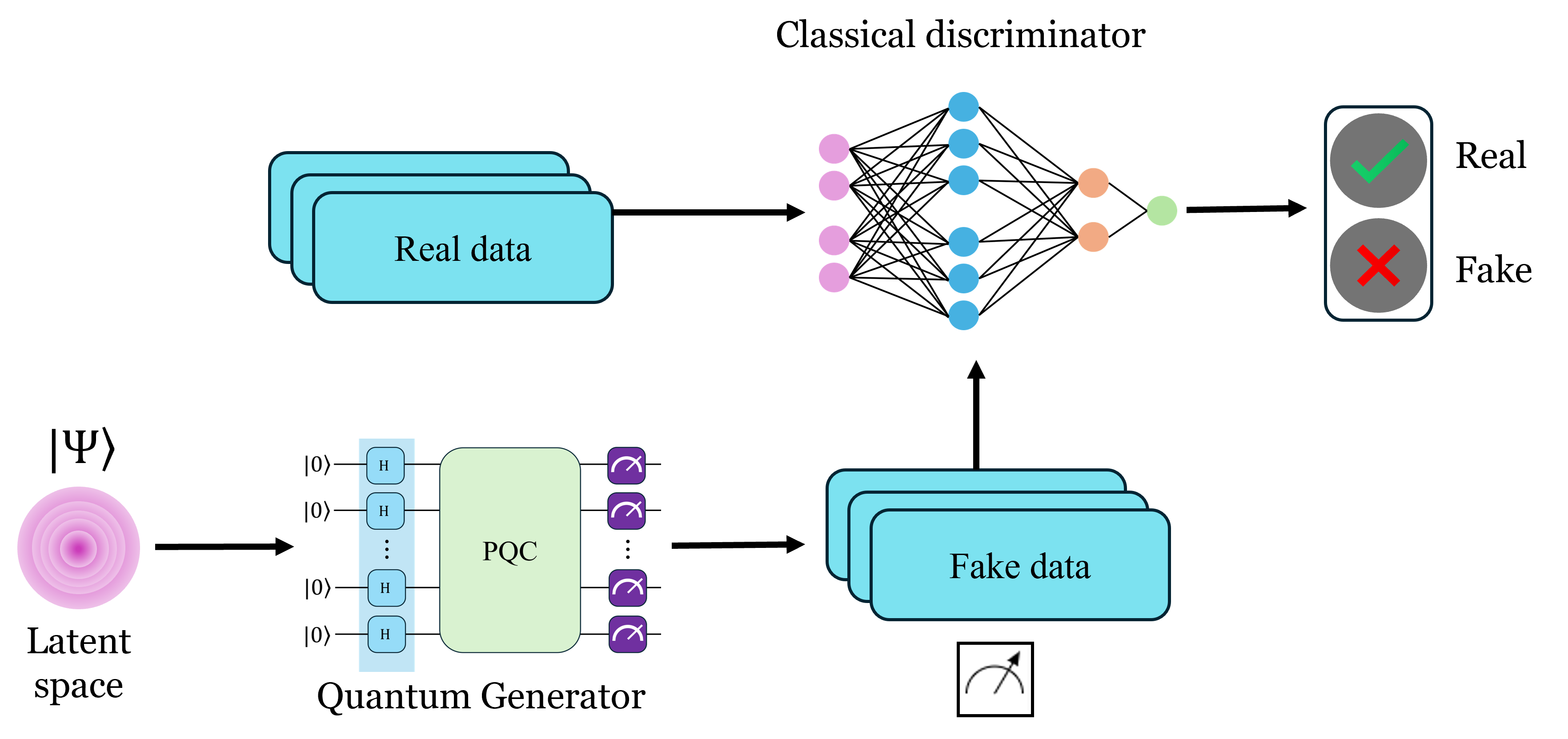
Quantum Generative Adversarial Networks (QGANs) represent a quantum extension of classical GANs, incorporating quantum mechanics to leverage the computational advantages of quantum systems [2] [3]. In QGANs, the generator is a parametrized quantum circuit that produces quantum states that resemble the distribution from the training data, meanwhile, the discriminator can be either a classical discriminator or a quantum parametrized circuit that differentiates between the training data distribution and generated distribution.

Simulating random variables with QGANs

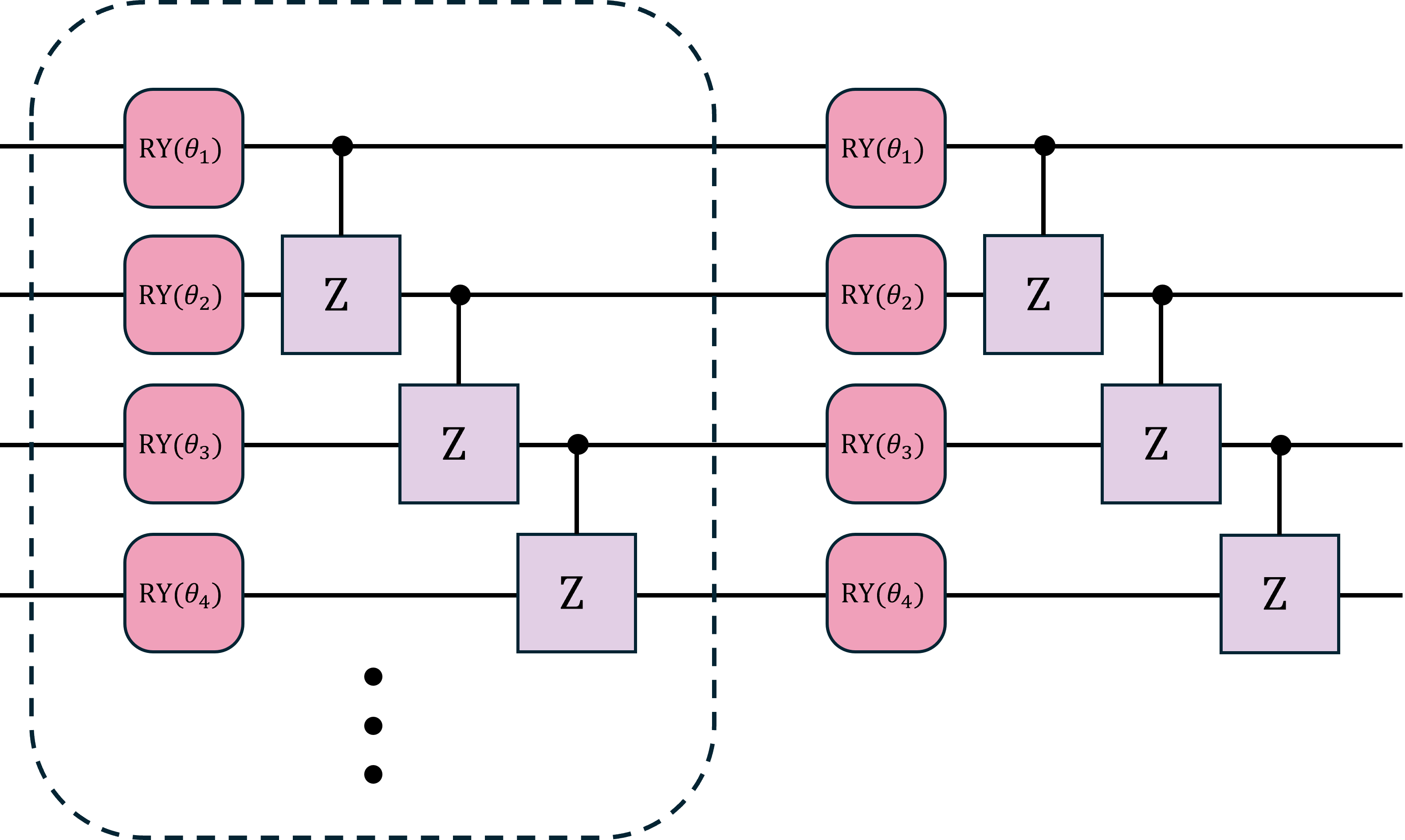
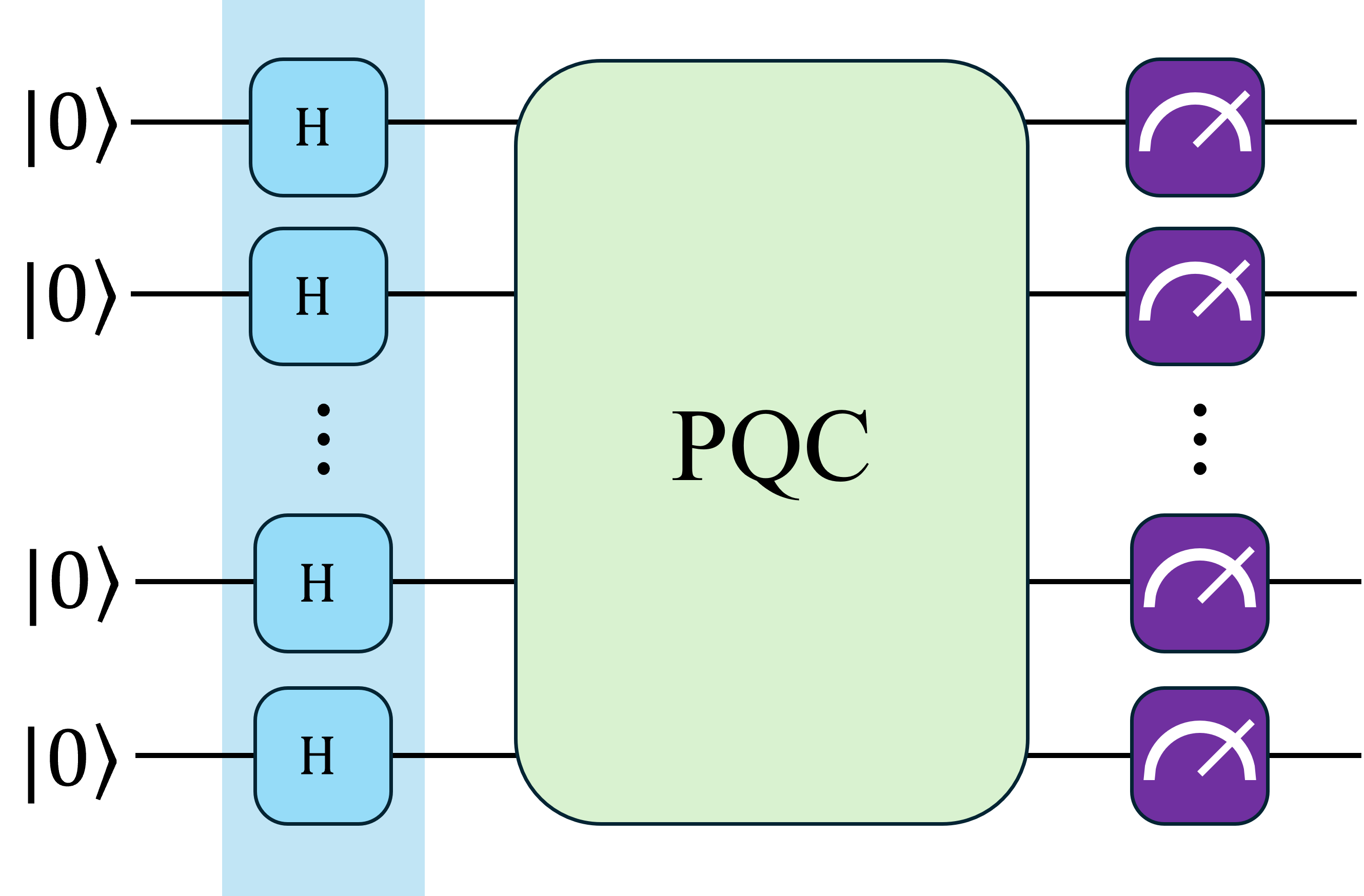
One of the key steps for the Monte Carlo Method is to specify the probability distribution of independent variables. An incorrect choice of the distribution can lead to inaccuracies. In my project, I try to address this difficulty by implementing QGANs for Monte Carlo Simulations. I used the architecture proposed by Zoufal et. al. [4], composed of a quantum generator with an equal superposition as a reference state followed by layers of parametrized \(\text{Pauli-Y}\) rotations followed by an entangling block of \(\text{control-Z}\) gates and a classical discriminator consisting of dense neural network.

a)

b)

The project implementation uses PennyLane and PyTorch. The generator circuit returns the probabilities of the basis states, each state representing a possible outcome. The circuit takes a weights parameter, as the name indicates, this parameter is an array with the angle of rotation of each parametrized \(\text{Pauli-Y}\) rotation.

dev = qml.device("default.qubit", wires=n_qubits)

@qml.qnode(dev, diff_method="backprop")
def quantum_circuit(weights):
    """Quantum generator's parametrized circuit"""

    weights = weights.reshape(q_depth, n_qubits)

    # Initialise latent vectors
    for i in range(n_qubits):
        qml.Hadamard(wires=i)

    # Repeat each layer
    for i in range(q_depth):
        # Parameterised layer
        for y in range(n_qubits):
            qml.RY(weights[i][y], wires=y)

        # Entangling blocks of control Z gates
        for y in range(n_qubits - 1):
            qml.CZ(wires=[y, y + 1])

        qml.Barrier(wires=list(range(n_qubits)), only_visual=True)

    return qml.probs(wires=list(range(n_qubits)))

The classical discriminator is a fully connected neural network with two hidden layers, containing 50 nodes in the first layer and 20 nodes in the second layer, both with a LeakyRelu activation function and, finally, an output layer of a single node with a sigmoid activation function to return the probability of an input to be a generated sample. The input layer shape depends on the number of possible outcomes the random variable of the training data can take. The discriminator's input is the pseudo-probabilities of a batch of samples from the random variable.

class Discriminator(nn.Module):
    """Fully connected classical discriminator"""

    def __init__(self):
        super().__init__()

        self.model = nn.Sequential(
            # Inputs to first hidden layer (num_input_features -> 50)
            nn.Linear(num_input_features, 50),
            nn.LeakyReLU(),

            # First hidden layer (50 -> 20)
            nn.Linear(50, 20),
            nn.LeakyReLU(),
            
            # Second hidden layer (20 -> 1)
            nn.Linear(20, 1),
            nn.Sigmoid(),
        )

    def forward(self, x):
        x = x.reshape(x.size(0), -1)
        
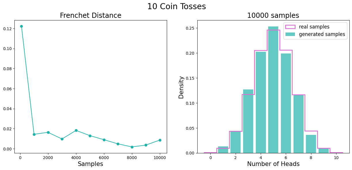
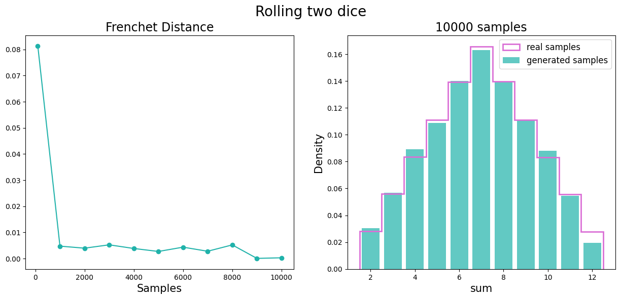
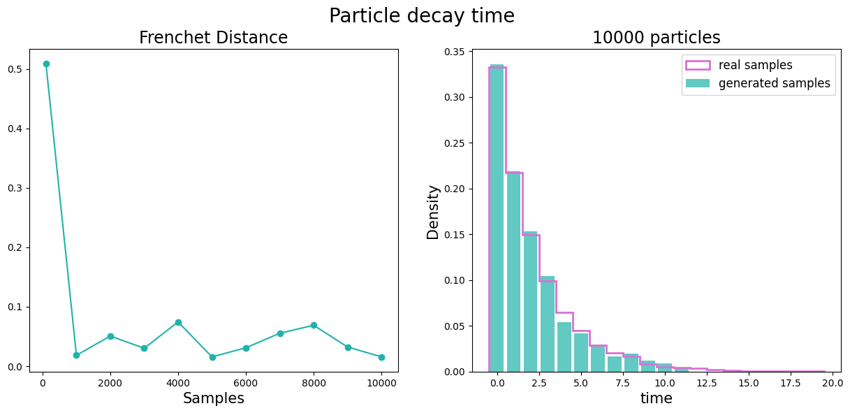
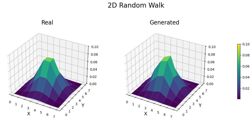
        return self.model(x)

I chose four simple scenarios to simulate: The rolling of two six-sided dice, coin toss sequences, particle time decay, and two-dimensional random walks. In this implementation, the quantum circuit returns the probability of measuring the elements in the basis state, and each element represents a possible outcome from the simulations. Once trained, the generator produces samples simulating a single event. The training process was the following:

• Data Generation
The training dataset was generated classically, composed of \(10^6\) samples for each scenario, and split into 1000 batches.
• Calculate Probabilities
The pseudo-probabilities of each batch were calculated and used to train the quantum generator, which returns the probabilities of each element in the basis state.
• Generator and discriminador
Two neural network models are defined. The discriminator is a classical neural network that tries to distinguish between real and fake data samples. At the same time, the generator is a quantum circuit designed to produce data samples that resemble the real data distribution.

a)

b)

c)

d)

Using a QGAN to generate gluon initiated jets

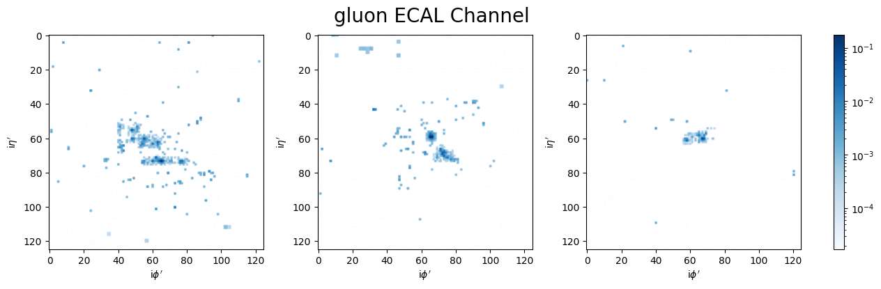
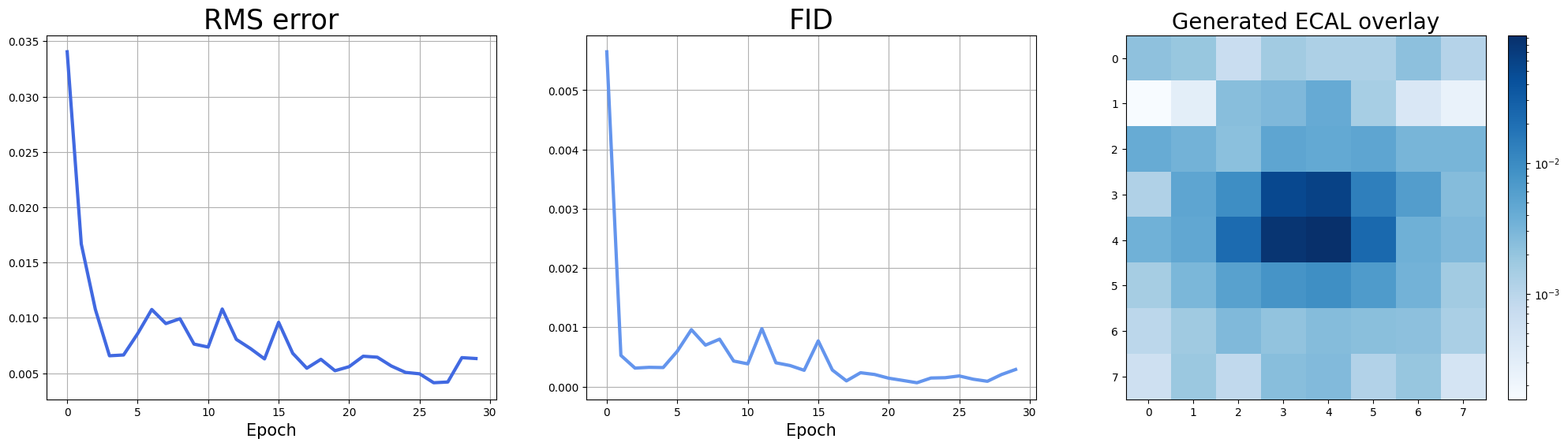
Moving to a more complex data distribution, I took the dataset of detector images from Quark-initiated jets [5]. Specifically, I used the electromagnetic calorimeter images that measure energy deposits from electromagnetic particles.

Due to the high complexity of the dataset, the first architecture was not powerful enough to resemble the training dataset distribution, which is why I implemented the architecture proposed by He Liang et. al.[6], which uses an auxiliary register to provide the PQC more possible solution states along with a post-processing step which allows the output of the quantum generator to get rid of the normalization constraint of the measurement. This architecture also uses many generators, each responsible for producing a fraction of the image. This approach allows each generator to focus on a simpler distribution rather than the more complex complete image.

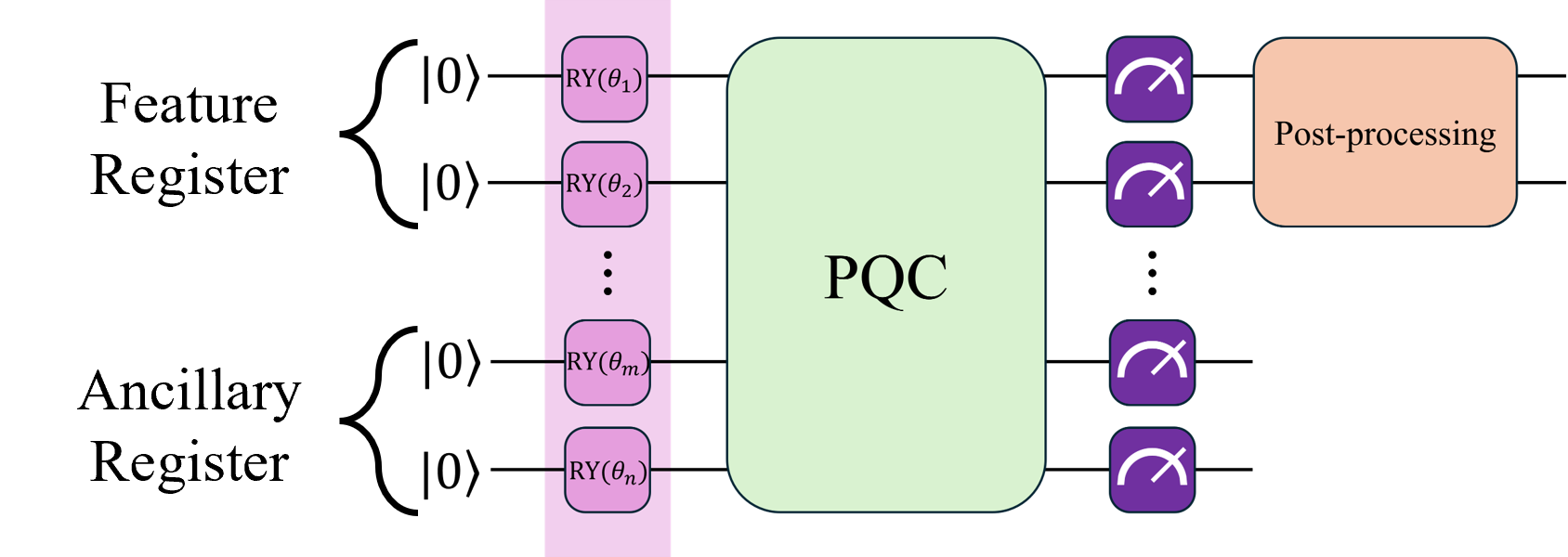
Quantum gates are unitary operators and, by definition, are linear transformations. With the most simple generative tasks like the examples from the section above, these transformations are good enough. However, for more complex data distribution, non-linear transformation could be needed. For the pre-measurement state of the generator, we have:

Where \(U_G(\theta)\) represents the overall unitary operator of the parametrized layers. If we take a partial measurement \(\Pi\) and trace out the ancillary subsystem:

The post-measurement state \(p(z)\), is dependent on \(z\) on the numerator and denominator. This implies a non-linear transformation was performed over \(|\Psi(z)\rangle\).

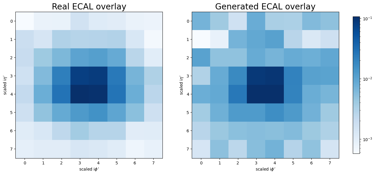
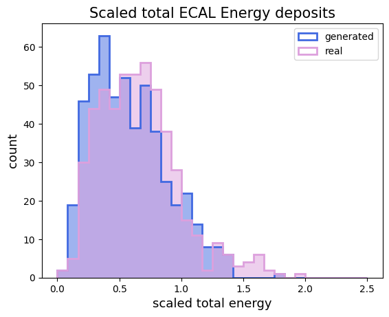
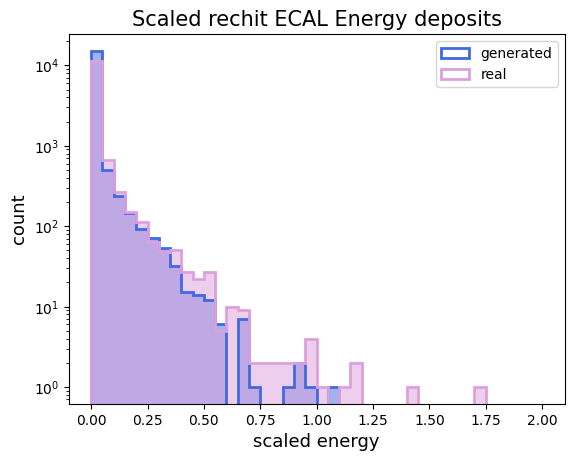
On the other hand, I wanted the output of the quantum generator to represent energy deposits, so the output should be able to take values larger than 1, and the elements from the quantum circuit output do not necessarily need to sum up to 1. These limitations can be overcome by applying the following transformation to the quantum circuit output of the circuit. \[ \tilde{x} = \frac{g}{y}\] Where \(g\) is the output from the generator and \(y \in (0, 1]\). In this work, I used, \(y=0.3\). The training process was the following:

• Data Preprocessing
From the ECAL channel, 512 images were down-scaled from \(125 \times 125\) to \(8 \times 8\) images using a sumpool transformation.
• Generator and discriminador
The model was trained during 30 epochs using a Stochastic Gradient Descent optimizer, the classical discriminator containing 50 nodes in the first layer and 20 nodes in the second layer, both with a LeakyRelu activation function and an output layer with a single node and sigmoid activation function. On the other hand, each of the two generators is a circuit with seven feature qubits, two auxiliary qubits, and ten layers.

a)

b)

a)

b)

Future work and conclusion

From the simple simulations and gluon-initiated jet image generation, we observe that implementing QGANs for data generation with simple and complex distributions is feasible. It would be interesting to investigate how well this implementation generates different yet correlated data distributions, such as the three subdetector channels from detector images [5]. The most exciting part of this project was exploring a promising method for future high-energy physics simulations. I am grateful for the opportunity to be part of the ML4SCI organization, their supportive community and cutting-edge projects are among the best I've encountered, inspiring people to pursue a career in this field. Thanks for your work.

References

[1] Ian J. Goodfellow, Jean Pouget-Abadie, Mehdi Mirza, Bing Xu, David Warde-Farley, Sherjil Ozair, Aaron Courville and Yoshua Bengio, Generative Adversarial Networks, arXiv:1406.2661v1.
[2] Pierre-Luc Dallaire-Demers, Quantum Generative Adversarial Networks, arXiv:1804.08641v2.
[3] Seth Lloyd, Christian Weedbrook, Quantum Generative Adversarial Learning, arXiv:1804.09139v1.
[4] Zoufal, C., Lucchi, A., & Woerner, S. (2019). Quantum Generative Adversarial Networks for learning and loading random distributions. Npj Quantum Information, 5(1). https://doi.org/10.1038/s41534-019-0223-2.
[5] Andrews, M., Alison, J., An, S., Bryant, P., Burkle, B., Gleyzer, S., Narain, M., Paulini, M., Poczos, B. & Usai, E. (2019). End-to-End Jet Classification of Quarks and Gluons with the CMS Open Data. Nucl. Instrum. Methods Phys. Res. A 977, 164304 (2020). https://doi.org/10.1016/j.nima.2020.164304.
[6] He-Liang, Yuxuan Du, Ming Gong, Youwei Zhao, Yulin Wu, Chaoyue Wang, Shaowei Li, Futian Liang, et. al. Quantum Generative Adversarial Networks for Image Generation, arXiv:2010.06201v3.